An R-package for analyzing natural language with transformers from HuggingFace using Natural Language Processing and Machine Learning.
The text-package has two main objectives:
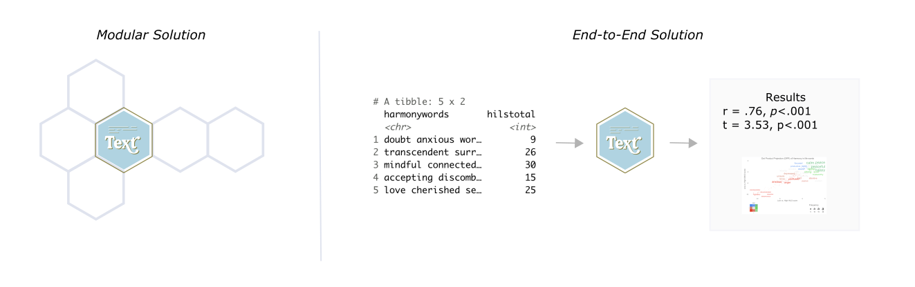
First, to serve R-users as a point solution for transforming text to state-of-the-art word embeddings that are ready to be used for downstream tasks. The package provides a user-friendly link to language models based on transformers from Hugging Face.
Second, to serve as an end-to-end solution that provides state-of-the-art AI techniques tailored for social and behavioral scientists.
Text is created through a collaboration between psychology and computer science to address research needs and ensure state-of-the-art techniques. It provides powerful functions tailored to test research hypotheses in social and behavior sciences for both relatively small and large datasets. Text is continuously tested on Ubuntu, Mac OS and Windows using the latest stable R version.
Please reference our tutorial article when using the package: The text-package: An R-package for Analyzing and Visualizing Human Language Using Natural Language Processing and Deep Learning.
Short installation guide
Most users simply need to run below installation code. For those experiencing problems or want more alternatives, please see the Extended Installation Guide.
For the text-package to work, you first have to install the text-package in R, and then make it work with text required python packages.
- Install text-version (at the moment the second step only works using the development version of text from GitHub).
GitHub development version:
# install.packages("devtools")
devtools::install_github("oscarkjell/text")
CRAN version:
install.packages("text")- Install and initialize text required python packages:
library(text)

# Install text required python packages in a conda environment (with defaults).
textrpp_install()

# Initialize the installed conda environment.
# save_profile = TRUE saves the settings so that you don't have to run textrpp_initialize() after restarting R.
textrpp_initialize(save_profile = TRUE)
Point solution for transforming text to embeddings
Recent significant advances in NLP research have resulted in improved representations of human language (i.e., language models). These language models have produced big performance gains in tasks related to understanding human language. Text are making these SOTA models easily accessible through an interface to HuggingFace in Python.
Text provides many of the contemporary state-of-the-art language models that are based on deep learning to model word order and context. Multilingual language models can also represent several languages; multilingual BERT comprises 104 different languages.
Table 1. Some of the available language models
| Models | References | Layers | Dimensions | Language |
|---|---|---|---|---|
| ‘bert-base-uncased’ | Devlin et al. 2019 | 12 | 768 | English |
| ‘roberta-base’ | Liu et al. 2019 | 12 | 768 | English |
| ‘distilbert-base-cased’ | Sahn et al., 2019 | 6 | 768 | English |
| ‘bert-base-multilingual-cased’ | Devlin et al. 2019 | 12 | 768 | 104 top languages at Wikipedia |
| ‘xlm-roberta-large’ | Liu et al | 24 | 1024 | 100 language |
See HuggingFace for a more comprehensive list of models.
The textEmbed() function is the main embedding function in text; and can output contextualized embeddings for tokens (i.e., the embeddings for each single word instance of each text) and texts (i.e., single embeddings per text taken from aggregating all token embeddings of the text).
library(text)
# Transform the text data to BERT word embeddings

# Example text
texts <- c("I feel great!")

# Defaults
embeddings <- textEmbed(texts)
embeddings
See Get Started for more information.
Language Analysis Tasks
It is also possible to access many language analysis tasks such as textClassify(), textGeneration(), and textTranslate().
library(text)

# Generate text from the prompt "I am happy to"
generated_text <- textGeneration("I am happy to",
                                 model = "gpt2")
generated_text
For a full list of language analysis tasks supported in text see the References
An end-to-end package
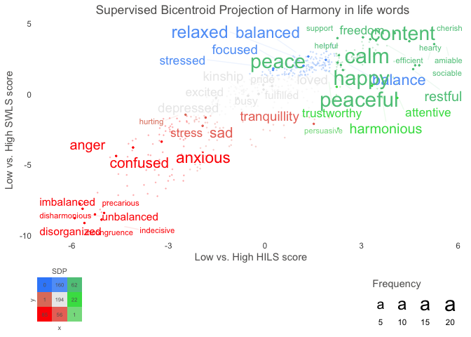
Text also provides functions to analyse the word embeddings with well-tested machine learning algorithms and statistics. The focus is to analyze and visualize text, and their relation to other text or numerical variables. For example, the textTrain() function is used to examine how well the word embeddings from a text can predict a numeric or categorical variable. Another example is functions plotting statistically significant words in the word embedding space.
library(text)
# Use data (DP_projections_HILS_SWLS_100) that have been pre-processed with the textProjectionData function; the preprocessed test-data included in the package is called: DP_projections_HILS_SWLS_100
plot_projection <- textProjectionPlot(
  word_data = DP_projections_HILS_SWLS_100,
  y_axes = TRUE,
  title_top = " Supervised Bicentroid Projection of Harmony in life words",
  x_axes_label = "Low vs. High HILS score",
  y_axes_label = "Low vs. High SWLS score",
  position_jitter_hight = 0.5,
  position_jitter_width = 0.8
)
plot_projection$final_plot