Plot words according to 2-D plot from 2 PCA components.
text2DPlot(
  word_data,
  min_freq_words_test = 1,
  plot_n_word_extreme = 5,
  plot_n_word_frequency = 5,
  plot_n_words_middle = 5,
  titles_color = "#61605e",
  title_top = "Principal Component Projection",
  x_axes_label = "Principal Component 1 (PC1)",
  y_axes_label = "Principal Component 2 (PC2)",
  scale_x_axes_lim = NULL,
  scale_y_axes_lim = NULL,
  word_font = NULL,
  bivariate_color_codes = c("#398CF9", "#60A1F7", "#5dc688", "#e07f6a", "#EAEAEA",
    "#40DD52", "#FF0000", "#EA7467", "#85DB8E"),
  word_size_range = c(3, 8),
  position_jitter_hight = 0,
  position_jitter_width = 0.03,
  point_size = 0.5,
  arrow_transparency = 0.1,
  points_without_words_size = 0.2,
  points_without_words_alpha = 0.2,
  legend_title = "PC",
  legend_x_axes_label = "PC1",
  legend_y_axes_label = "PC2",
  legend_x_position = 0.02,
  legend_y_position = 0.02,
  legend_h_size = 0.2,
  legend_w_size = 0.2,
  legend_title_size = 7,
  legend_number_size = 2
)
Arguments
| word_data | Dataframe from textPCA |
|---|---|
| min_freq_words_test | Select words to significance test that have occurred at least min_freq_words_test (default = 1). |
| plot_n_word_extreme | Number of words that are extreme on dot product projection per dimension. (i.e., even if not significant; per dimensions, where duplicates are removed). |
| plot_n_word_frequency | Number of words based on being most frequent. (i.e., even if not significant). |
| plot_n_words_middle | Number of words plotted that are in the middle in dot product projection score (i.e., even if not significant; per dimensions, where duplicates are removed). |
| titles_color | Color for all the titles (default: "#61605e") |
| title_top | Title (default " ") |
| x_axes_label | Label on the x-axes. |
| y_axes_label | Label on the y-axes. |
| scale_x_axes_lim | Manually set the length of the x-axes (default = NULL, which uses ggplot2::scale_x_continuous(limits = scale_x_axes_lim); change e.g., by trying c(-5, 5)). |
| scale_y_axes_lim | Manually set the length of the y-axes (default = NULL; which uses ggplot2::scale_y_continuous(limits = scale_y_axes_lim); change e.g., by trying c(-5, 5)). |
| word_font | Font type (default: NULL). |
| bivariate_color_codes | The different colors of the words (default: c("#398CF9", "#60A1F7", "#5dc688", "#e07f6a", "#EAEAEA", "#40DD52", "#FF0000", "#EA7467", "#85DB8E")). |
| word_size_range | Vector with minimum and maximum font size (default: c(3, 8)). |
| position_jitter_hight | Jitter height (default: .0). |
| position_jitter_width | Jitter width (default: .03). |
| point_size | Size of the points indicating the words' position (default: 0.5). |
| arrow_transparency | Transparency of the lines between each word and point (default: 0.1). |
| points_without_words_size | Size of the points not linked with a words (default is to not show it, i.e., 0). |
| points_without_words_alpha | Transparency of the points not linked with a words (default is to not show it, i.e., 0). |
| legend_title | Title on the color legend (default: "(DPP)". |
| legend_x_axes_label | Label on the color legend (default: "(x)". |
| legend_y_axes_label | Label on the color legend (default: "(y)". |
| legend_x_position | Position on the x coordinates of the color legend (default: 0.02). |
| legend_y_position | Position on the y coordinates of the color legend (default: 0.05). |
| legend_h_size | Height of the color legend (default 0.15). |
| legend_w_size | Width of the color legend (default 0.15). |
| legend_title_size | Font size (default: 7). |
| legend_number_size | Font size of the values in the legend (default: 2). |
Value
A 1- or 2-dimensional word plot, as well as tibble with processed data used to plot..
See also
see textProjection
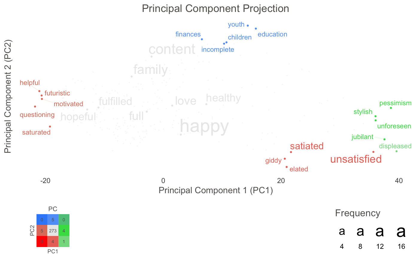
Examples
# The test-data included in the package is called: DP_projections_HILS_SWLS_100 # Dot Product Projection Plot principle_component_plot_projection <- text2DPlot(PC_projections_satisfactionwords_40) principle_component_plot_projection#> $final_plot#> #> $processed_word_data #> # A tibble: 292 x 13 #> words n Dim_PC1 Dim_PC2 check_extreme_m… check_extreme_m… #> <chr> <int> <dbl> <dbl> <dbl> <dbl> #> 1 acce… 1 -11.4 4.79 0 0 #> 2 acco… 2 -10.3 7.52 0 0 #> 3 achi… 1 3.08 17.1 0 0 #> 4 acti… 1 -3.79 8.28 0 0 #> 5 adeq… 1 -7.50 8.40 0 0 #> 6 alive 1 2.25 -1.43 0 0 #> 7 alone 1 8.31 -3.75 0 0 #> 8 ambi… 1 -8.43 -4.33 0 0 #> 9 amus… 1 11.8 -4.24 0 0 #> 10 anal… 1 2.28 6.42 0 0 #> # … with 282 more rows, and 7 more variables: check_extreme_min_PC1 <dbl>, #> # check_extreme_min_PC2 <dbl>, check_extreme_frequency <dbl>, #> # check_middle_PC1 <dbl>, check_middle_PC2 <dbl>, extremes_all <dbl>, #> # colour_categories <chr> #>names(DP_projections_HILS_SWLS_100)#> [1] "words" "dot.x" #> [3] "p_values_dot.x" "n_g1.x" #> [5] "n_g2.x" "dot.y" #> [7] "p_values_dot.y" "n_g1.y" #> [9] "n_g2.y" "n" #> [11] "n.percent" "N_participant_responses"